
Cyclistic Mobility Case Study
Interactive Vizualization - GitHub Repo
Overview
I was tasked with developing 12 months of real-world urban bike-sharing data (5.8 million rows) into actionable insights for a fictional company called Cyclistic.
- Technology: SQL, Tableau
- Timeline: 1 week
- Role: Data Analyst
- Date Completed: July 2023
Scenario
You are a data analyst working in the marketing analyst team at Cyclistic, a bike-share company in Chicago. The director of marketing believes the company’s future success depends on maximizing the number of annual memberships. Therefore, your team wants to understand how casual riders and annual members use Cyclistic bikes differently. From these insights, your team will design a new marketing strategy to convert casual riders into annual members. But first, Cyclistic executives must approve your recommendations, so they must be backed up with compelling data insights and professional data visualizations.
The Business Task
Identify how casual riders and annual members use Cyclistic bikes differently.
The Data
Data Source: This analysis uses 12 months of anonymized, first-party trip data (June 2022 – May 2023) provided by Divvy. The full raw dataset and monthly CSV files are made publicly available by the City of Chicago and can be accessed here.
Columns:
- ride_id
- rideable_type
- started_at
- ended_at
- start_station_name
- start_station_id
- end_station_name
- end_station_id
- start_lat
- start_lng
- end_lat
- end_lng
- member_casual
After downloading and organizing the data, we will need to combine all 12 months into a single dataset.
First, I will clear any previous attempts:
DROP TABLE IF EXISTS all_trips;
Then, I will combine the data into a new table
CREATE TABLE IF NOT EXISTS all_trips AS
SELECT * FROM '202206_divvy_tripdata'
UNION ALL
SELECT * FROM '202207_divvy_tripdata'
UNION ALL
SELECT * FROM '202208_divvy_tripdata'
UNION ALL
SELECT * FROM '202209_divvy_publictripdata'
UNION ALL
SELECT * FROM '202210_divvy_tripdata'
UNION ALL
SELECT * FROM '202211_divvy_tripdata'
UNION ALL
SELECT * FROM '202212_divvy_tripdata'
UNION ALL
SELECT * FROM '202301_divvy_tripdata'
UNION ALL
SELECT * FROM '202302_divvy_tripdata'
UNION ALL
SELECT * FROM '202303_divvy_tripdata'
UNION ALL
SELECT * FROM '202304_divvy_tripdata'
UNION ALL
SELECT * FROM '202305_divvy_tripdata';`
Now, I check to see if it worked – it did:
SELECT * FROM all_trips;
Next, I check the total number of rows in the dataset:
SELECT COUNT(*) FROM all_trips;
There are 5,829,030 rows of data.
Processing the Data
First, I will check the data for any duplicate entries
SELECT COUNT(ride_id) - COUNT(DISTINCT ride_id) AS duplicates
FROM all_trips;
Finding no duplicates, I check each column for any empty cells:
-- To detect empty cells:
SELECT COUNT(*) FROM all_trips WHERE ride_id == '';             -- 0
SELECT COUNT(*) FROM all_trips WHERE rideable_type == '';       -- 0
SELECT COUNT(*) FROM all_trips WHERE started_at == '';          -- 0
SELECT COUNT(*) FROM all_trips WHERE ended_at == '';            -- 0
SELECT COUNT(*) FROM all_trips WHERE start_station_name == '';  -- 834,545 empty cells detected
SELECT COUNT(*) FROM all_trips WHERE start_station_id == '';    -- 834,677 empty cells detected
SELECT COUNT(*) FROM all_trips WHERE end_station_name == '';    -- 891,757 empty cells detected
SELECT COUNT(*) FROM all_trips WHERE end_station_id == '';      -- 891,898 empty cells detected
SELECT COUNT(*) FROM all_trips WHERE start_lat == '';           -- 0
SELECT COUNT(*) FROM all_trips WHERE start_lng == '';           -- 0
SELECT COUNT(*) FROM all_trips WHERE end_lat == '';             -- 5,961 empty cells detected
SELECT COUNT(*) FROM all_trips WHERE end_lng == '';             -- 5,961 empty cells detected
SELECT COUNT(*) FROM all_trips WHERE member_casual == '';       -- 0
Finding nearly 1M empty cells, I will be sure to filter them.
But first, I’ll check the length of each ride_id to verify consistency and accuracy:
SELECT DISTINCT(LENGTH(ride_id)) FROM all_trips;
All ride_id values are 16 characters long without exception.
Next, I will check how many different values for member_casual there are, ensuring there are no invalid entries.
SELECT DISTINCT(member_casual) FROM all_trips;
Finding no typos here, I will do the same for rideable_type.
SELECT DISTINCT(rideable_type) FROM all_trips;
Next, I will be creating a new column which provides a ride_length for each entry:
SELECT
    started_at,
    ended_at,
    ROUND(((JULIANDAY(ended_at) - JULIANDAY(started_at)) * 1440), 2) AS ride_length
FROM all_trips;
After creating the ride_length column, I can check for any ride lengths that may be invalid:
SELECT COUNT(ride_length)
FROM
    (SELECT
        started_at,
        ended_at,
        ROUND(((JULIANDAY(ended_at) - JULIANDAY(started_at)) * 1440), 2) AS ride_length
    FROM all_trips)
WHERE ride_length < 0 OR ride_length > 1440;
I have detected 5,397 entries with a ride length of less than 0 or greater than 24hrs. These will be filtered out in the next step.
Data Cleaning
Taking what we have learned in the previous stage, I will be creating a new table that filters out inaccurate or incomplete data, and calling it cleaned_trips. This table will also include new columns: ride_length, weekday, month, and start_hour.
First, I will clear any previous attempts at creating this new table:
DROP TABLE IF EXISTS cleaned_trips;
Next, creating the new table:
CREATE TABLE IF NOT EXISTS cleaned_trips AS
    SELECT *,
        ROUND(((JULIANDAY(ended_at) - JULIANDAY(started_at)) * 1440), 2) AS ride_length,
        CASE CAST (STRFTIME('%w', started_at) AS INTEGER)
            WHEN 0 THEN 'Sunday'
            WHEN 1 THEN 'Monday'
            WHEN 2 THEN 'Tuesday'
            WHEN 3 THEN 'Wednesday'
            WHEN 4 THEN 'Thursday'
            WHEN 5 THEN 'Friday'
            WHEN 6 THEN 'Saturday' END AS weekday,
        CASE CAST (STRFTIME('%m', started_at) AS INTEGER)
            WHEN 1 THEN 'January'
            WHEN 2 THEN 'February'
            WHEN 3 THEN 'March'
            WHEN 4 THEN 'April'
            WHEN 5 THEN 'May'
            WHEN 6 THEN 'June'
            WHEN 7 THEN 'July'
            WHEN 8 THEN 'August'
            WHEN 9 THEN 'September'
            WHEN 10 THEN 'October'
            WHEN 11 THEN 'November'
            WHEN 12 THEN 'December'
            END AS month,
        SUBSTR(started_at, 12,2) AS start_hour
    FROM all_trips
    WHERE start_station_name <> ''
        AND start_station_id <> ''
        AND end_station_name <> ''
        AND end_station_id <> ''
        AND end_lat <> ''
        AND end_lng <> '';
This new table has 4,494,681 rows, meaning 1,334,349 entries have been removed before analysis.
Data Engineering Workflow
To ensure accuracy across nearly 6 million records, I implemented a multi-stage ETL (Extract, Transform, Load) process:
- Data Consolidation: Used UNION ALL to aggregate 12 separate CSV files into a unified relational table for analysis.
- Data Cleaning: Conducted a comprehensive audit for null values and duplicates. I removed approximately 1.3M incomplete entries to ensure high-confidence reporting.
- Feature Engineering: Created time-series variables (ride_length, weekday, start_hour) using SQL date functions to transform raw timestamps into usable dates.
Data Analysis
Before diving deep into the data, I will create a few tables that show the dataset at a glance.
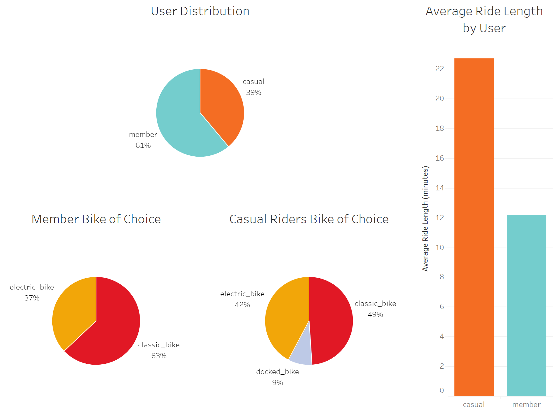
First, a table that shows the breakdown of users:
SELECT member_casual, COUNT(member_casual) AS total_trips
FROM cleaned_trips
GROUP BY member_casual;
Next, a table that shows the breakdown of bike types being used by each user type:
SELECT rideable_type, member_casual, COUNT(rideable_type) AS total_rides
FROM cleaned_trips
GROUP BY member_casual, rideable_type;
A table showing the average ride length of each user type:
SELECT member_casual, AVG(ride_length) AS average_ride_length
FROM cleaned_trips
GROUP BY member_casual;
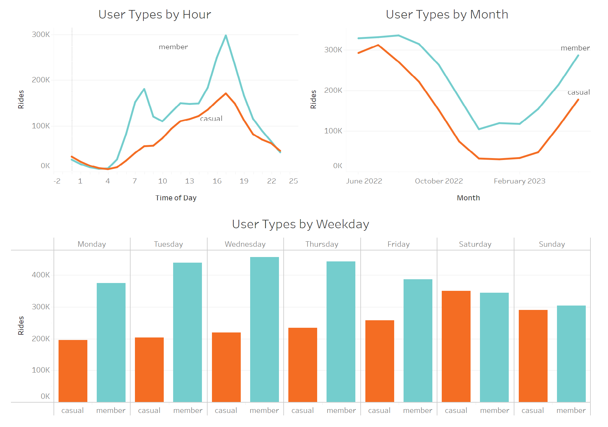
Now, I will be taking a look at when both user groups use Cyclistic bikes, starting by breaking it down by hour:
SELECT member_casual, start_hour, COUNT(start_hour) AS total_rides
FROM cleaned_trips
GROUP BY member_casual, start_hour;
Now, breaking down ridership by weekday for both groups:
SELECT member_casual, month, COUNT(month) AS total_rides
FROM cleaned_trips
GROUP BY month, member_casual
ORDER BY member_casual, started_at;
Finally, showing when rides are taken by month:
SELECT member_casual, month, COUNT(month) AS total_rides
FROM cleaned_trips
GROUP BY month, member_casual
ORDER BY member_casual, started_at;
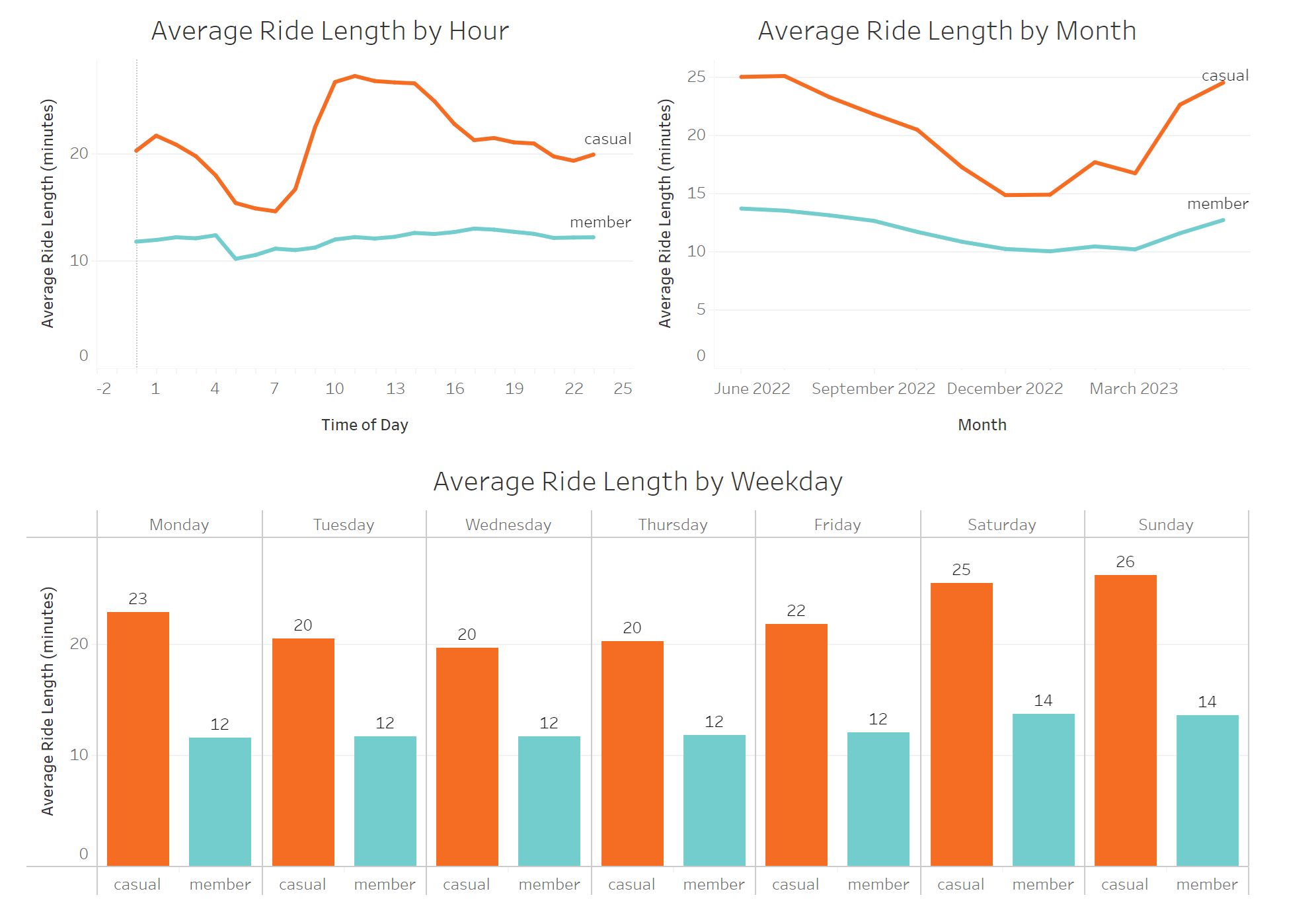
Now that we know how ridership differs over time, we will take a look at how long each user type uses a bike, on average.
First, checking hourly breakdown of ride length:
SELECT member_casual, start_hour, AVG(ride_length) AS average_ride_length
FROM cleaned_trips
GROUP BY start_hour, member_casual
ORDER BY member_casual, start_hour;
Next, average ride length by weekday:
SELECT member_casual, weekday, AVG(ride_length) AS average_ride_length
FROM cleaned_trips
GROUP BY weekday, member_casual
ORDER BY member_casual, started_at;
And now, average ride length by month:
SELECT member_casual, month, AVG(ride_length) AS average_ride_lenth
FROM cleaned_trips
GROUP BY month, member_casual
ORDER BY member_casual, started_at;
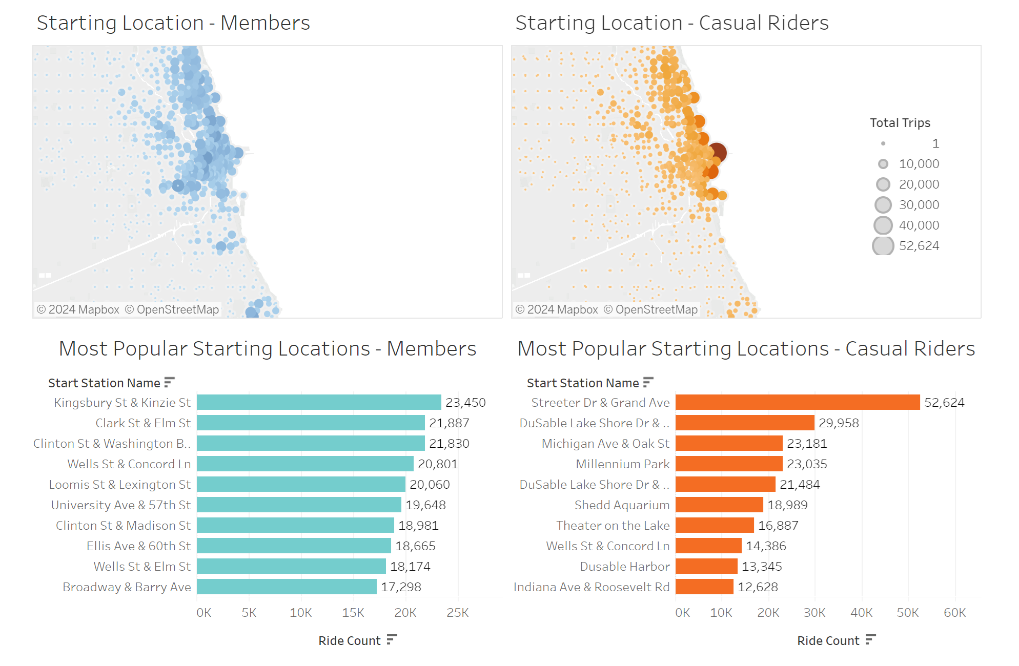
Now that we have looked at when rides are taken and for how long, we will take a look at where.
I’ll create a top ten list for the most popular starting stations, first for members:
SELECT start_station_name, COUNT(ride_id) AS start_station_total
FROM cleaned_trips
WHERE member_casual = 'member'
GROUP BY start_station_name
ORDER BY start_station_total DESC
LIMIT 10;
Then, for casual riders:
SELECT start_station_name, COUNT(ride_id) AS start_station_total
FROM cleaned_trips
WHERE member_casual = 'casual'
GROUP BY start_station_name
ORDER BY start_station_total DESC
LIMIT 10;
Now, I will create a table that pairs each of the starting locations by name, and assigning them to a latitude and longitude. This is done by averaging latitude and longitudinal values, establishing the coordinates of each individual station.
SELECT start_station_name, member_casual,
  AVG(start_lat) AS start_lat,
  AVG(start_lng) AS start_lng,
  COUNT(ride_id) AS total_trips
FROM cleaned_trips
GROUP BY start_station_name, member_casual
ORDER BY member_casual, total_trips DESC;
Now that we’ve gained some important insights on our data, it’s time to create visuals and insights on everything we’ve learned so far.
Data Visualized
See my interactive vizualization here
Key Findings
- We see a significant influx of member rides at 8 am and 5 pm, indicating that members tend to rely on Cyclistic bikes for their daily commute.
- In contrast, casual riders are most active on weekends, suggesting that casual riders tend to use the service for leisure.
- On average casual users’ average ride length is close to double that of members, supporting the hypothesis that casual riders’ routes are more meandering, slower, or less purpose-driven compared to members, who are likely commuting.
- Casual riders predominantly start their rides near Chicago’s center of tourism, whereas members exhibit a more diverse starting location preference, which tends to be farther away from the city center. This finding further strengthens the distinction between commuters and sight-seers among the two user types.
Recommendations
Based on the findings listed above, there is a fundamental difference in the purpose of rides taken by both user groups. These purposes must be taken into account when developing marketing campaigns to convert casual riders into members.
- Develop a new “Weekend Pass” product. This could be a new membership type that caters to the casual riders’ existing habits of riding on the weekends. This creates a middle ground for prospective members and will generate recurring revenue from the casual rider group.
- Develop marketing materials that focus on the potential for commuting. Casual riders may not have ever considered using the bikes for anything other than leisure, and advertisements highlighting this possibility could make the difference.
- In order to target the casual rider, we can use the data to determine when and where to reach them:
- Between the months of March and October, when Cyclistic is used the most.
- During the weekends, when casual riders are most active.
- Near Streeter Dr & Grand Ave, by far the most popular station used by casual riders.